XXX ASCII file storage on AWS S3
XXX ASCII file storage began on Unix filesystems
Back from the 1990s all the XXX ASCII raw and processed data was stored on Unix filesystems. This was typically mounted onto hosts from an NFS share that was served up either by another Unix host, or by a NAS appliance.
The ASCII files were stored compressed, first using the SunOS native compress format, and then later switching to the more modern gzip format. Since the file suffix .Z is used by compress, this influenced some naming conventions, with some files still carrying forward the .Z suffix even though they are now actually gzipped files.
The folder structure in use for the last 20 years has 2 roots:
/data/vendors/for non-client-specific raw and processed files, and/data/clients/for client-specific raw and processed files
AWS migration switched XXX from NAS to S3
In the Xxxxxxx datacenter we were storing /data/vendors/ and /data/clients/ on very expensive NetApp NAS appliances. When we migrated to AWS, we were able to take advantage of the ability of a Linux host to mount an AWS S3 bucket as a Linux native filesystem to swap out the NAS appliances for S3 buckets and reduce our ASCII storage costs by a factor of 10 or so.
On each Linux host, filesystems are normally mounted using the /etc/fstab file. We went from having a line that looked like this (mounting a Xxxxxxxxxx NetApp share):
xxxnhppnns0030v.xxxxxxx.net:/vol/xxx1_data1/vendors /data/vendors nfs vers=3,nodev,proto=tcp,intrto a line that looks like this (mounting an S3 bucket):
s3fs#xxx-ascii /data/vendors fuse allow_other,_netdev 0 0
Navigating through the /data/vendors (and /data/clients) subtrees on the Linux host looks exactly the same whether the mount comes from an expensive NAS appliance or from S3. All Unix filesystem semantics are preserved, which is extremely important because all our C code and ASCII processing scripts were written assuming that the files live on a Unix filesystem.
How S3 stores files
S3 is a hierarchical object store and its hierarchical key structure does map well to a directory structure, but S3 does not know that it is storing Unix-type files as its objects. What makes our Unix file storage on S3 possible is that every object stored in S3 can have arbitrary metadata attached to it. Here is the AWS S3 console view of the file /data/vendors/xxxxxxx/201912/ww/raw/20191201.ven=xxx.type=ww.rows=733138.Z. See it storing the uid, gid and Unix file mode; the mode includes the permissions and the type of file (in this case, it's a symbolic link):

The Linux host interprets the metadata and hierarchical key of each object and transforms these into the normal Unix file/directory semantics.
Athena queries against files on S3
What's Athena?
Athena is a managed implementation of the PrestoDB software package that was opensourced by Facebook. PrestoDB is a SQL query engine that can be pointed to many different data sources and formats. AWS added the ability for PrestoDB to use S3 as a source of data, and several different object formats on S3 are supported.
Public Athena
The standard Athena product is a serverless service that runs on some unknown pool of AWS managed hosts that are all shared by any customer that is executing Athena queries. Our queries only have permission to go against our own S3 buckets as data sources. Since this unknown pool of hosts is managed by AWS, we only pay per query, but as we know, our queries can fail due to lack of resources, perhaps caused by contention with whatever other queries customers are running.
Private Athena
AWS has for a long time had an instant-cluster product call EMR. AWS has packaged a lot of software pre-installed on these clusters, and this includes PrestoDB. All a customer has to do is to specify what kind of servers they want and how many servers they want, and a cluster with PrestoDB can automatically spring to life, pointing to our S3 buckets as data sources. Once we have the cluster IP, we can send SQL queries to it the same as we can send queries to Athena, and this way very large queries can run very quickly. But we pay for every minute of uptime for every server in the cluster.
What kind of files can be queried?
When you define a table in Athena, you tell it:
- the table layout (columns and their data types)
- the location in S3 where the objects you want to query are
- the format of these objects.
Here are some formats Athena understands:
Super fast Parquet
Parquet is a read-only columnar compressed indexed format which is comparable to the kinds of internal data files created by DBMS systems like Oracle, DB2 or Redshift. There are ways to convert ASCII files to Parquet files and once that's done, Athena queries against those files can be really fast, because Athena can quickly locate and read only that part of the specific Parquet file which is required by a query.
Data can be spread across multiple Parquet files, and these files can be spread across multiple S3 key/paths for partitioning.
CSV and JSON
Athena can also natively query plain old CSV and JSON files, but you don't want to store a LOT of data in this format because Athena has to plow through each file until it finds what your query is looking for. It does some caching, but it's still slow. If you have a lot of data in these formats, you can let Athena convert it to Parquet format using a "create table as select" statement, telling Athena that the new table you are creating will use Parquet format.
If the files are compressed, Athena can decompress them while reading them.
ASCII files defined by regular expressions
This is intended for things like web server log files where certain patterns indicate specific data elements. But we can use this for querying our ASCII data files by just defining a single column per table (the column could be named "row") and defining a single regex (.*) that grabs all the characters on a line for our single column. Once we have a row, we can use SQL string functions to extract substrings based on column positions.
This access is also slow, but we would only access the data this way ONCE, against the raw input data, in order to use a "create table as select" statement to ETL-copy the data into a new Parquet format table.
Just like with CSV and JSON files, if the files are compressed, Athena can decompress them while reading them.
We are not bound to Athena
As long as the raw file rows can be loaded into a SQL database, this same processing flow can be followed. The one advantage to Athena is that the raw file rows are automagically available for SQL queries without having to load them into any database. In some different environment, the downstream steps would be the same after the initial raw file rows were loaded.
Process flow
Using C programs
Only certain data at certain points in the process flow is available to be queried this way.

Using SQL scripts
All the data is always available for query, through both Athena and Redshift. Fixed width ASCII file deliveries can be continued by using SQL string functions to create query outputs with the field widths and formatting needed for continuity of file deliveries to customers.

Running a series of linked views instead of one giant SQL statement
This idea showed up in a couple of places:
- Hotels.com wrote an article in Medium about this
- The Apache Foundation has a Confluence page on this topic
The point is that rather than having a large, highly nested and complex SQL statement to achieve your result, instead you break your query up into a sequence of linked views that each select from the prior view. Each view represents one logical step of your ETL process flow. This gives you the same end result as nesting the SQL but it creates an environment where each step of the logic can be tested individually by applying little unit test queries against each view.
To obtain your final result you just select from the final view in your series of views, which pulls from the prior view, which pulls from the prior view, ...etc..
This arrangement is especially useful if you can do the following things:
- Put the views under version control
- Interactively browse the results of each step-view during the development process (like viewing data structures in a running C program using gdb)
- Halt your production processing with an ab-end if a unit test against one of the views fails
You get all that for free with Jupyter notebooks
Embedding scripts in Jupyter notebooks
Here is an example of how clear code looks when mixed with documentation in a Jupyter notebook:

- A notebook is a JSON file. Its content is a sequence of cells like spreadsheet cells, except that each cell can contain code from a multitude of languages, including SQL, or it can contain rich documentation in HTML or Markdown, enabling the "literate programming" environment envisioned by Donald Knuth.
- You edit a notebook in your web browser, connecting your browser to a Jupyter server.
- While editing the notebook in your browser, you can interactively change and execute the code in each cell, and the output (if any) of each cell's execution is displayed below the cell.
- There's a HUGE ecosystem of web-widgets that let you display, sort, scroll through, search through, and chart and graph your data, etc. This lets a developer graphically verify the data, AND if desired, the charts and widgets can be embedded into the notebook and updated with each production batch run.
- The Jupyter server can check your notebook into a git version control repository, display diffs between your current version and the head version in git, and can save your notebook as a JSON file into your home directory on the server, or let you download the notebook through your browser.
- The notebook can be saved or checked-in WITH the current outputs of cell executions, or WITHOUT any cell outputs. This actually allows test cases to be embedded in the code check-in.
- Jupyter can export a notebook as HTML or PDF, creating instant reports. In many cases, the HTML can have embedded interactive charts and data widgets, with the data residing in JSON stored inside the HTML file. This file you are reading is an HTML export of a notebook. The cells in this notebook contain only (automatically) numbered documentation.
- The notebook can be executed in batch mode, running the code cell by cell unless an error causes it to ab-end.
Notebooks in the clouds
Notebooks elsewhere
- LIGO shares their black hole research via notebooks; a quote from an article in The Atlantic Magazine "The Scientific Paper Is Obsolete. Here's what's next": The paper announcing the first confirmed detection of gravitational waves was published in the traditional way, as a PDF, but with a supplemental [Jupyter] notebook.
- "Jupyter is the new Excel"
- "All the cool kids are doing it"
- QuantStack, CloudQuant, Quantopian - Jupyter is very popular on Wall Street
- InfoWorld: Data analysis made easier
Revision control
With one click on a toolbar button, you can perform a version control checkin of the notebook currently being edited:

Graphical diffs
With one click on a toolbar button, graphical diffs can be shown between a developer's current working copy and their own last saved version, or between their own last saved version and the version checked in to the version control repository:

Checkin history
A click of another toolbar button will display the commit history of the notebook being edited:

Executing notebooks in batch mode
Only cells with the tag "batch" will be executed
Each cell can have multiple tags applied to it for many purposes; for example, during editing, a filter can be applied in the web browser to only view cells with tags matching a pattern that you supply.
You can freely include all kinds of very heavy development code, or table widgets or even embedded full-blown spreadsheets or 3D visualization widgets, etc. and as long as those cells don't have the tag "batch", they will not get executed.
However, cells with HTML/Markdown documentation will never be excluded regardless of their tags.
Command line arguments
A cell with the tag "parameters" will have its values overridden by command line arguments. This means that you can define fixed values of variables (like proc date, or GDS code) in a cell at the top of your notebook for development, but during production these values will be dynamically set by command line arguments.
Log files
- When you execute a notebook in batch mode, the process starts by automatically creating a copy of the notebook with all the cell outputs blanked out (in case the notebook was saved with any current cell outputs).
- Then as each cell executes, its output is inserted (as normally happens in a live notebook in your web browser) just below the code cell that created the output.
- If an error occurs while executing a cell, execution stops after that cell's output is inserted.
- The batch run produces:
- the output notebook (which is a json file)
- along with a text-only-log version
- along with an HTML export of the notebook
These are all available for examination after a batch run for information that would normally be gotten from a log file.
Example lines from the text-only-log file
Parts of XX and XX processing are running as Jupyter notebooks in batch mode. Here is an example of the text-only log, which is has a format very similar to our current runcmd logs:
Managing and scheduling notebook execution via Apache Airflow
We have a Jupyter server installed on our ASCII-code development machine in AWS. That is a medium sized Linux machine, but that's OK because it's horsepower is only used for the process of serving up notebooks to web browsers for editing and display, not for running notebooks in batch mode.
The other tool we need for running notebooks in batch mode is called Apache Airflow. It schedules notebooks, monitors them for timely success or failure, initiates automatic retries, keeps track of dependencies between jobs, displays dashboards of jobs in progress, and sends alerts if needed.
Another tool that all the cool kids are using...
Started by AirBNB, and also taken up by PayPal and eBay, it has a lot of information and momentum.
Companies using this include: Adobe, AirBNB, AirDNA, Bloomberg, Capital One, eBay, Etsy, Glassdoor, Groupon, HBO, HotelQuickly, Los Angeles Times, Logitravel, Lyft, Overstock, Pandora, PayPal, Quantopian, SnapTravel, Spotify, Square, Tesla, The Home Depot, Twitter, United Airlines, Yahoo
Google is offering it as a managed service
Cost savings using AWS EC2 spot instances
Although all the heavy lifting will be done by whatever executes the SQL (public Athena, private Athena, Redshift, Oracle, etc.), Airflow will execute each notebook on a fresh dedicated inexpensive EC2 spot instance of whatever size is specified to avoid having all notebooks running on a single-point-of-failure server.
Also, isolating each notebook to a newly instantiated dedicated server with a lifecycle that only exists during the runtime of the job insures that there can be no interference or state dependencies between any code.
Tracking and reporting features
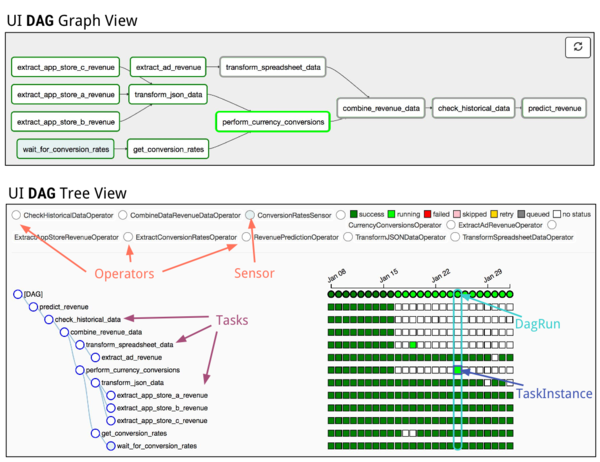
Airflow lets you structure notebook batch runs into tree-like DAGS (directed acyclic graphs) which match the patterns we have implemented over the years using scripts calling other scripts in directory hierarchies.
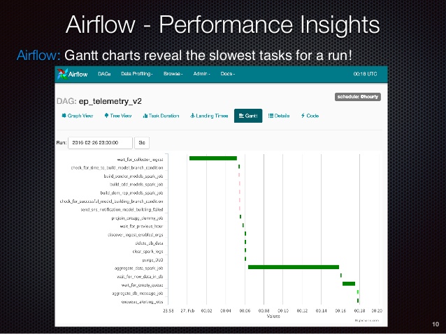
Screenshots from other companies
Here are some screenshots from the internet showing that other people use Airflow to do exactly the same kinds of ETL work as we do:
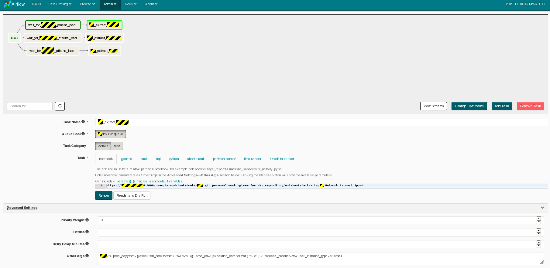
Screenshots from our implementation
Parts of XX processing are running as Jupyter notebooks invoked by Airflow on EC2 spot instances executing SQL against Athena.
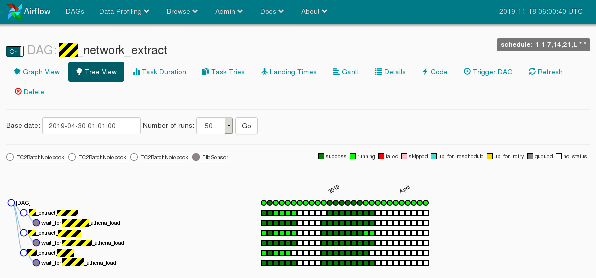
Here is the workflow editor where the XX_network_extract DAG is constructed:
Comes with many useful plugins for handling cloud data tasks
One of the most useful being a plugin that allows for "create partition as select" operations on Athena/PrestoDB tables, so that you can save the results of your ETL flows by just doing a "select * from final_view" using the idea of a series of linked views.
This idea of only modifying tables partition-by-partition is what we've been doing with Oracle for 20 years, and it's very popular right now.
Allows easy processing in parallel environments
You can set up any number of dev/qa/prod environments, and easily get your environment name in your notebook so that you can parameterize schema names, or table names or S3 locations. Once a notebook version makes it to production, nothing in it would have to change as long as the code was parameterized with the environment name.
Good integration with the AWS console
The AWS console can display the currently running Airflow/Jupyter notebook batch EC2 spot instances by job and task name:

AWS Cost Explorer can break down costs by job and task name:
